Expression gradient analysis
In this workflow, the spatial expression gradient between two reference regions are created. The distances are renormalised such that results from different images can be more easily be compared.
As input the workflow requires:
- FISH-quant results file: created with FISH-quant.
- ImJoy annotation files: annotations of the two reference regions.
Summary of analysis workflow
The expression gradient is calculated as follows
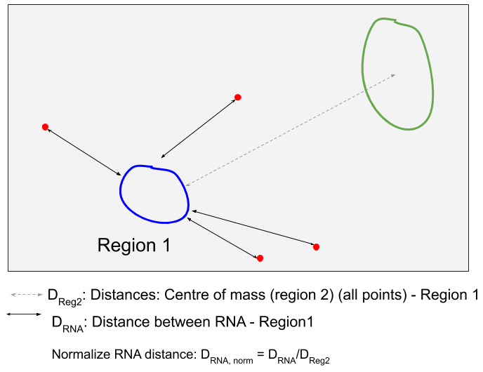
- In the analysis, the distance for RNA from the first reference region is calculated (the shortest distance between the RNA and the polygon defining this region). Negative distances mean that the RNA is inside, positive that the RNA is outside.
-
These distances are then renormalised with the shortest distance between the center of mass of the second region and the polygon of the first region.

-
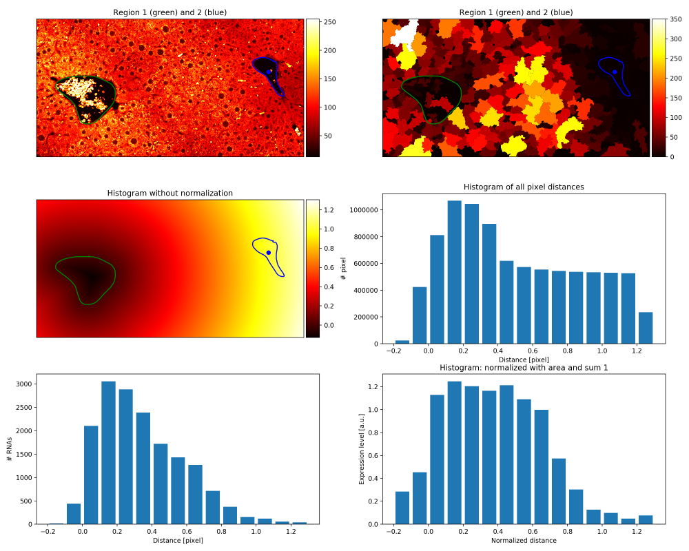
Distances are then summarised in histograms with bins of width 0.1 between the minimum and maximum renormalised distance measurements.
- These counts are then further renormalised to consider the actual contained area in the image for a given distance. This is done by calculating the distance transform of the image with respect to region 1. These values are treated distance measurements, and treated as described for the RNA distance measurements. The obtained histogram counts are used to normalise the RNA distance counts.
- Lastly, the histogram is such that frequencies sum up to 1.
Required tools
ImJoy Plugins
These plugins have to be installed only once, after installation they will be
available in the dedicated ImJoy workspace: liver-rna-loc
Pressing on the links below, will open ImJoy in your browser (best in Chrome) and allow you to install the required plugins. You will be asked to confirm the installation with a dialog as shown below. After confirmation, the plugins will be installed together with additional auxiliary plugins.
-
ImageAnnotator: annotate your images. Install from here. -
ExpGradient: calculate expression gradient. Install from here.

Jupyter notebook
To perform the calculation of the expression gradients, we also provide a
Jupyter notebook expression_gradient.ipynb, which can be found on GitHub
in the folder notebooks.
Data
Data organisation
This workflow requires that data is organised in the following away
- A parental folder contains all sample folders, e.g.
data__expression_gradientfor the example data. - Each sample (usually a field of view) is in a separate folder, e.g. named
sample_1,sample_2, .... Each sample folder can contain images of multiple channels. - FQ result file are in the same folder. A folder can contain FQ results for different channels.
- An annotation file with the two reference regions (
annotation.json). See below for more details.
In the example below, a folder contains the annotations (annotation.json),
two different channels (...(green).tif and ...(red).tif ), the FQ results
for both channels ....txt, and an annotation file (annotation.json).
Please note that you can have only one annotation file per sample folder. You can generate it based on any of the channels, but the same annnotations will be used for each FQ results file in this folder.
├─ data__expression_gradient/
│  ├─ sample_1
│  │  ├─ annotation.json
│  │  ├─ sample_1_green_outline_spots_181018.txt
│  │  ├─ sample_1_green.tif
│  │  ├─ sample_1_red_outline_spots_181017.txt
│  │  ├─ sample_1_red.tif
│  ├─ sample_2
│  │  ├─ ...
Demo data
You can find already processed demo data here.
TODO: upon publication, demo data will be moved to Zenodo.
Analysis
1. RNA detection with FQ
Please consult the dedicated section here for more details.
2. Annotation of reference regions
Please consult the dedicated section here for more details.
For this workflow, you need TWO different annotations
- Central vein, we recommend naming it
CV. - Portal lobe, we recommend naming it
PL.
3. Calculate density profiles
You can run this analysis either with the provided code in the Jupyter notebook, or use ImJoy.
Analysis in ImJoy
If you use ImJoy, you need to install the Python plugin engine. The first installation might take a bit of time, since the necessary Python environments are created.
Once installed, you will see in the the plugin in the sidebar. Before using it, you have to specify the labels of the two reference regions. To access the plugin parameters, press on the arrow down symbol next to the plugin name.
In the example below the labels CV and PL are defined for the first and second
region, respectively.

Then you can press on the plugin name to execute the plugin. In a dialog, you will be asked to specify a folder, please select the parental folder containing the different sample folders. The plugin will then analyse all sample folders containing an annotation file. The regions in this file will then be used to establish the spatial expression gradient between these two regions.
Progress is reported in the plugin log (accessible with the 'i' symbol next to the plugin name) and the ImJoy progress bar.
With Jupyter notebook
Once you have your conda environment installed as described in the Overview section, you can open the Jupyter notebook and analyze your data. You have to execute the first cell to load the necessary code.
The second cell allows you to
- Define the folder containing your data.
- Defining the labels for the two annotated reference regions.
Executing the cell, will launch the analysis workflow. described above.
4. Generated result files
The function will create a number of result files, which are stored in the
subfolder analysis__exprGradient.
Results files have the full name of the FQ file with the following prefixes
-
_summary_density (PNG file). Contains plots of expression density plots. Cells are filled with pixel values corresponding to their expression level.
-
_summary_gradient (PNG file). Contains summary plots for the spatial gradients between two the two reference points (the first plot shown on this page).
-
hist_expression (tab delimited text file). Contains the spatial expression gradient as a table:
- 1st col: normalised distance,
- 2nd col: normalised counts by number of pixels (4th col)
- 3rd col: RNA counts
- 4th col: number of pixels in the image within range (for normalisation)
-
img_density (16bit tif file). Contains the expression density plots. The pixel value of the cell corresponds to the number of RNAs in this cell. No outlines are shown. Files can be rendered with Fiji and an adequate look-up table.
-
img_density_outline (16 bit tif file). Contains the expression density plot and the cell outlines. The outlines of the cells are set to the maximum RNA count in the image. This guarantees that the outlines can be seen.
-
img_outline (8 bit image). Outlines of all cells in the image.